‍

1. Introduction

Over the past few years, pre-trained models have fundamentally reshaped expectations for what data-driven models can achieve in language, vision, and video applications. That playbook is by now familiar: pre-train on large, curated datasets, then adapt through fine-tuning. The question is whether it can deliver the same transformative gains in industrial engineering, when the objective is predicting physical behavior on complex geometries and when every ground-truth example must be generated through expensive high-fidelity simulation rather than scraped from the web.

At PhysicsX, we are building Large Physics Models (LPMs) that give a positive answer to that question. LPMs accelerate the design optimization and inverse design workflows that drive industrial engineering value. Unlike surrogate models built from scratch for every new problem, pre-trained LPMs reach high accuracy on new use cases with far less simulation data.

In our previous post, we introduced the PhysicsX Data Factory and PXNetCar — a proprietary dataset of 20K+ industrial RANS simulations across 250+ baseline vehicles, with morph variants exploring aerodynamically meaningful design changes. We also flagged a key evaluation challenge: widely used public datasets like DrivAerNet++ and Luminary SHIFT-SUV cover a narrow set of design families, so held-out test metrics are easy to over-interpret. Models may appear to generalize, yet remain brittle when applied to new vehicle families or solver regimes.

In this post, we introduce PX-Car-Aero-v1, our latest state-of-the-art pre-trained LPM for automotive external aerodynamics, trained on an expanded PXNetCar dataset: now 444 baselines, making a total of over 33,000 simulated designs after incorporating morphed variations. PX-Car-Aero-v1 is built on PX Transformer Neural Field, our custom transformer-based architecture that predicts scalar forces (i.e., drag and lift) alongside surface and volumetric fields — crucially, without requiring an expensive volumetric computational fluid dynamics (CFD) mesh at inference.

We demonstrate that fine-tuning a pre-trained LPM on a realistic, previously unseen dataset achieves the same performance as a simulation surrogate model trained from scratch while requiring ~80% less data. Notably, this advantage holds even in cross-simulator settings, where the model must adapt to a different simulation configuration using only a small number of fine-tuning simulations — a particularly challenging scenario we highlighted in our previous post. We also find that this advantage grows as the design space expands: surrogate models trained from scratch require progressively more simulation data to maintain performance, while fine-tuned LPM achieve comparable accuracy with a roughly fixed data budget.

These benefits also compound over time. Fine-tuned accuracy follows clear data scaling laws in the size of the pre-training corpus; as PXNetCar grows, the same modest fine-tuning budget steadily delivers better results.

PX-Car-Aero-v1 is now available on the PhysicsX platform, enabling engineering teams to fine-tune and deploy their own LPMs using only a small amount of simulation data from their own vehicle designs, with minimal additional data and compute requirements.

A follow-up post will dive deeper into the architecture, benchmarking, and the key design decisions behind PX-Car-Aero-v1.

‍

2. PX-Car-Aero-v1

2.1 Expanded PXNetCar

Since our last post, the PhysicsX Data Factory has been continuously generating automotive geometries and simulations for our pre-trained models and experiments. The PXNetCar dataset now includes 444 unique baselines and a median of 88 morphed variants per baseline, resulting in 33,203 unique automotive simulations.

The simulations employ the RANS k-omega SST turbulence model with an inlet velocity of 30 m/s, which provides a good balance between the accuracy needed for common engineering design use cases and computational efficiency. Each geometry and simulation is then verified for convergence and physical realism.

The expanded dataset further increases coverage across car types and overall geometric diversity.

2.2 PX-Car-Aero-v1 Architecture

The architecture of PX-Car-Aero-v1 is a custom geometry-context field-query transformer, which takes as input a surface geometry and optionally volumetric points, and outputs:

• Scalar forces: coefficients of drag and lift (Cd, Cl, respectively);
• Surface fields: pressure coefficient and wall shear stress (WSS) coefficient;
• Volumetric fields: pressure coefficient and normalized velocity.

We note that Cd and Cl can also be calculated by computing the force integral of the pressure and WSS, which we call Integrated Cd and Integrated Cl below.

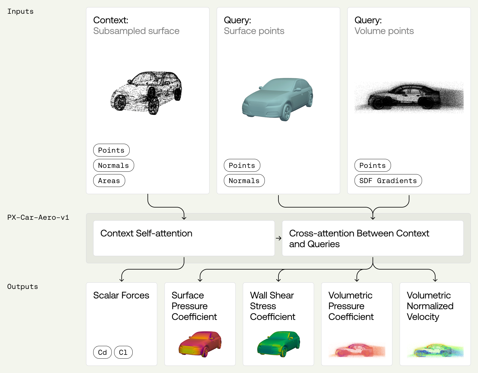
The architecture consists of three streams: surface context, surface queries, and volume queries. The surface context stream builds a latent representation of the geometry via an initial geometry context encoding layer and subsequent self-attention blocks. These blocks are interleaved with cross-attention branches for surface and volume queries.

The model architecture shares the same broad transformer pattern as AB-UPT (Alkin et al., 2025). The differences to AB-UPT, as well as the Transolver architecture we used previously, are user-focused:

• Relaxed inference-time requirements. Both surface and volumetric fields can be predicted at arbitrary points or none at all. In particular, unlike architectures such as Transolver or Point Cloud Transformer, our architecture doesn’t require a volumetric CFD mesh at inference time, eliminating a preprocessing step that can take orders of magnitude longer than inference itself. For applications that require only scalar predictions, the query streams can be omitted entirely.
• Efficient scaling to an arbitrary number of predicted query points. By separating and caching the surface context stream, we can process an arbitrary number of queries in chunks, generating consistent field predictions on the full set of query points. This approach is faster than the method used in Transolver-3 (Zhou et al., 2026).
• Surface mesh invariance. The surface context stream has low sensitivity to the meshing of the surface it accepts as input, eliminating the need for expensive CFD-grade preprocessing. This is made possible by applying quadrature weights whenever the network aggregates information across surface points.

2.3 A Strong Pre-trained Starting Point

On common public benchmarks, DrivAerNet++ and DrivAerML, the PX Transformer Neural Field architecture is competitive with the best published results. Trained on our own PXNetCar data, PX-Car-Aero-v1 is highly accurate on designs from the regions it has already seen.

On genuinely new designs, while there is degradation in accuracy across all metrics, the quantities that matter most for engineering — above all, the direction of an incremental change in scalar forces — are the ones that hold up best. Moreover, zero-shot out-of-distribution accuracy follows clear data scaling laws, improving consistently as we grow the model and data size.

To further improve the accuracy of the PX-Car-Aero-v1 model on a new design, we can fine-tune it with a small amount of data, which is what we focus on in the following section.

‍

3. Adapting PX-Car-Aero-v1 to Industrial Use Cases

Every real-world automotive engineering problem comes with its own vehicle family, design space, and simulation setup. The natural baseline is therefore a bespoke surrogate, trained from scratch on proprietary high-fidelity simulation data. Generating the simulation data is the dominant cost, so the question becomes whether a pre-trained LPM reduces that cost by providing a better starting point.

Our results show that it does. In typical engineering scenarios, fine-tuning PX-Car-Aero-v1 requires approximately 80% less simulation data than training the same architecture from scratch to achieve the same level of performance. Crucially, this saving holds even when the user's simulations come from a solver that the model never saw during pre-training. This enables a single pre-trained model to serve different contexts and solver setups, rather than being tied to the one it was originally trained on.

Further, the broader and more complex the design space, the greater the advantage over training from scratch. This is the benefit of pre-training on a diverse set of geometries: the model adapts to a wide design space with a realistic simulation budget.

In the following sections, we compare fine-tuning the pre-trained PX-Car-Aero-v1 on the target dataset with training the same architecture from scratch — starting from randomly initialized weights and learning exclusively from the target data. Both approaches use identical training procedures after initialization, with no method-specific tuning, identical train-validation splits, and a small held-out validation set for early stopping.

3.1 Fine-tuning a Pre-trained Model Requires ~80% Less Data than Training from Scratch

The first use case we investigate is a production-grade SUV (Vehicle A) morphed across a 21-parameter space and simulated under detached eddy simulation (DES). This is the furthest setup from our pre-training, since it asks the model to simultaneously absorb a geometry shift and a solver shift. The 21 parameters cover both structural changes, such as overhangs, roof height and curvature, and front fascia, as well as finer detail changes, such as ride height, wheel, tyre, and diffuser geometry.

The figures below sweep the full range of fine-tuning data budgets, doubling at each step. Each budget is reported as a train + validation split (e.g., 20+5), where the validation set is used for early stopping. Because the validation simulations must also be generated, they are included in the total simulation budget. We repeat the whole sweep over three random splits to guard against random effects. Within each split, we hold out a fixed test set of unseen car designs and grow the budgets by nested sub-sampling, so that larger budgets are supersets of smaller ones. Each budget is evaluated on its own held-out test set, rather than a single shared set of designs. The reported curves show the mean across the three train-validation splits, while the shaded bands indicate the minimum and maximum performance across those splits.

Across these sweeps, we track the following metrics:

• Integrated CD directional accuracy measures, across all pairs of design variants, how often the model correctly predicts the direction of a change in drag.
• Delta Integrated CD MAE (mean absolute error) is the absolute difference between the average absolute difference between the predicted and true change in drag when moving from one design variant to another.
• Finally, field RL2 (relative L2 error) measures how closely a predicted field matches the true field across every point simultaneously. It is computed as the Frobenius norm of the difference between the predicted and true fields, divided by the Frobenius norm of the true field.

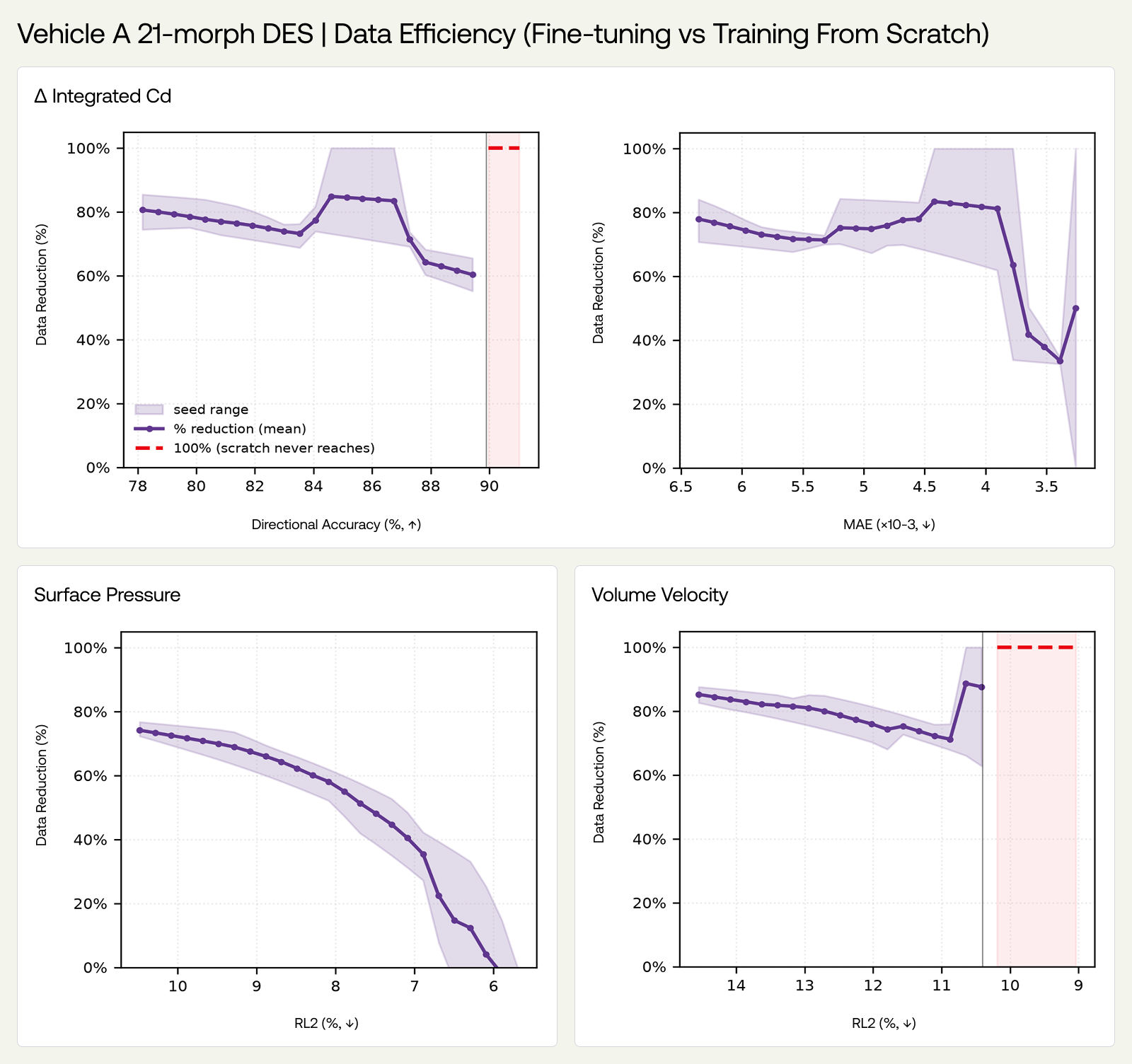
Fine-tuning shows a clear and consistent advantage over training from scratch. At a modest budget of just 25 simulations (a 20+5 train-validation split), fine-tuning reliably ranks designs, achieving a Cd directional accuracy of 85.6%, compared with 68.3% for the same architecture trained from scratch.

The other three metrics tell the same story at that budget: fine-tuning leads by ~50%. The gap is even more pronounced at the smallest data budget: with just a 5+2 train-validation split, fine-tuning achieves a directional accuracy of 76.8%, while training from scratch remains near-random at 51.9%. As expected, the gap begins to close at a high simulation budget. At lower data budgets, the fine-tuned model also exhibits less variation across trials on drag-related metrics than the model trained from scratch.

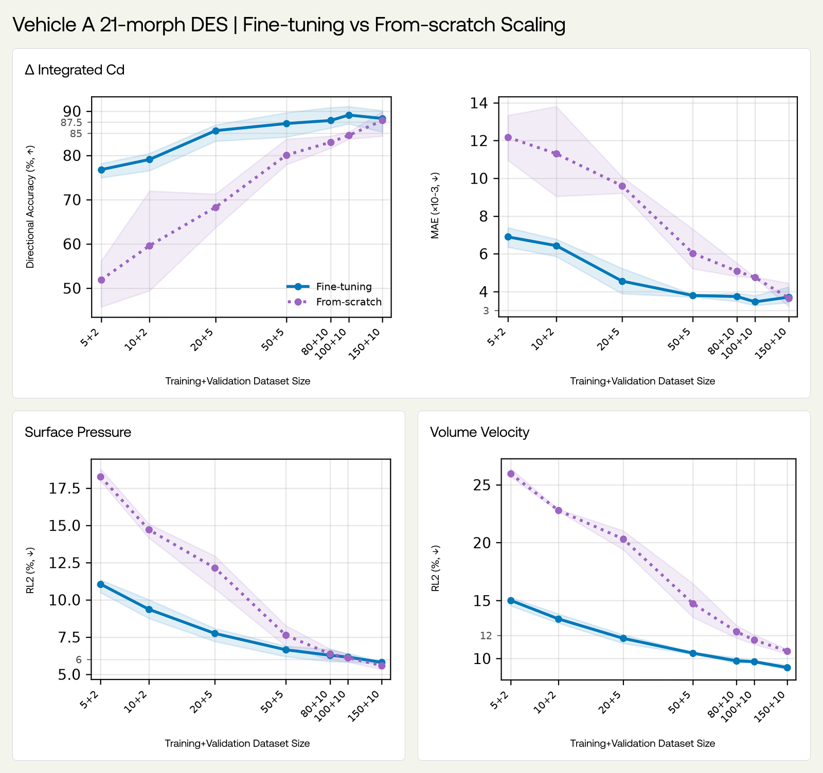
Framed in terms of data efficiency — that is, the reduction in simulation data required to achieve a given level of accuracy — fine-tuning delivers an approximately 80% reduction in simulation requirements across a wide range of performance levels. For a directional accuracy of at least 85%, fine-tuning requires roughly 84.4% fewer simulations; at a target directional accuracy of at least 90%, training from scratch does not reach the threshold at any of the data budgets evaluated, whereas fine-tuning does. The same picture holds on volume velocity RL2: the saving sits at 75-86% across the mid-range of targets, and fine-tuning reaches the tightest volume-velocity accuracies (below 10% RL2) that training from scratch never clears within the swept budget.

Altogether, this translates into a substantial reduction in simulation data generation costs, which typically dominate the overall cost of model development. Fine-tuning also offers a secondary benefit: faster training. At a given dataset size, both approaches require approximately the same time per epoch, but training from scratch requires ~1.75× more epochs on the 20+5 split (while still failing to reach the target performance). As a result, fine-tuning reaches the 0.85 threshold in under one-tenth of the wall-clock time.

3.1.1 This holds on independent third-party data: DrivAerML

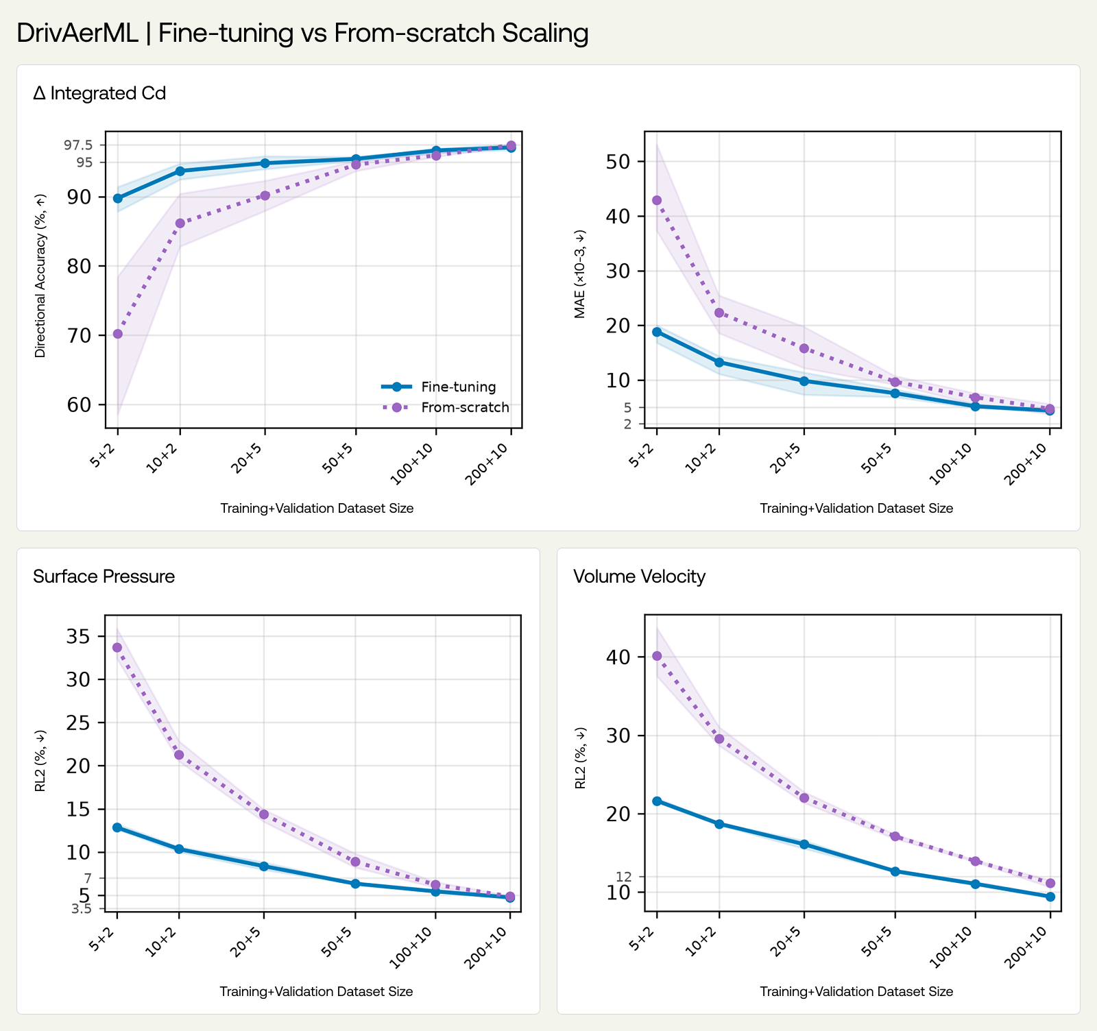
DrivAerML is an independent, third-party DES dataset that carries none of our own geometry or pipeline choices, so it serves as a clean external check. In this example, we fix the test set to the official 48-sample split from the GeoTransolver paper and randomize only the fine-tuning subset across seeds. The fine-tuned model is useful from the smallest budgets: at the 20+5 split, it already ranks designs at a directional accuracy of about 95%, a surface-pressure RL2 of 8.4%, and a volume velocity RL2 of 16.1%. Training from scratch starts well behind, at 70% against 90% for fine-tuning at the 5+2 split, and climbs steeply. It catches fine-tuning on ranking by the 50+5 split, while on delta CD MAE, surface-pressure RL2, and volume velocity RL2, fine-tuning still leads by 14-32% relative at 100+10.

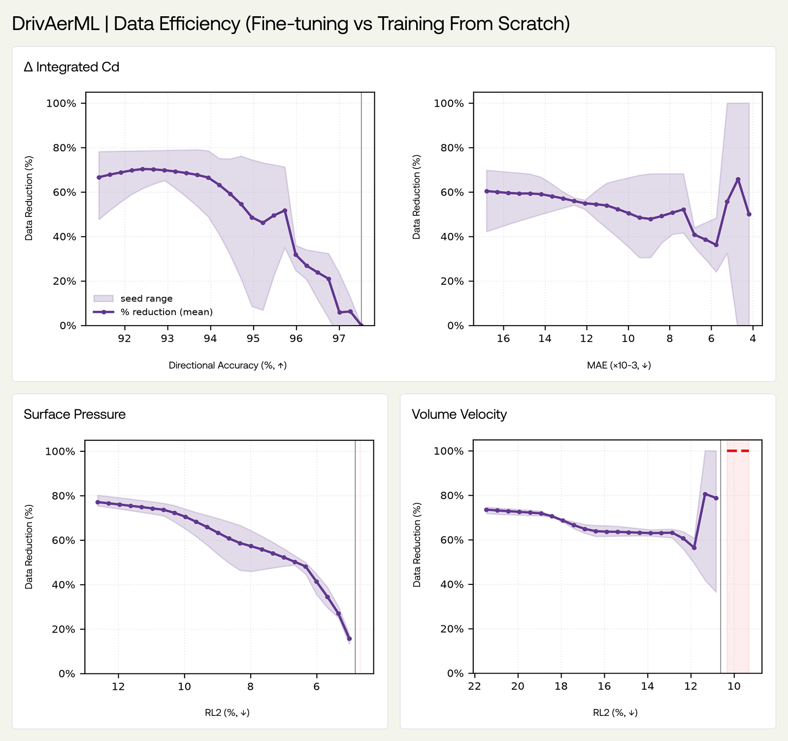
The pre-training advantage is therefore largest where it matters most for a user: at the low- and mid-data budgets that drive the simulation cost decision. Expressed in terms of data efficiency — that is, the reduction in simulations required to reach the same performance target — fine-tuning reduces the simulation budget by 30-70% across the range of targets it achieves.

‍

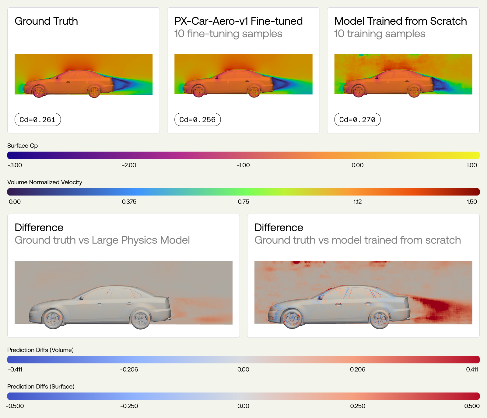
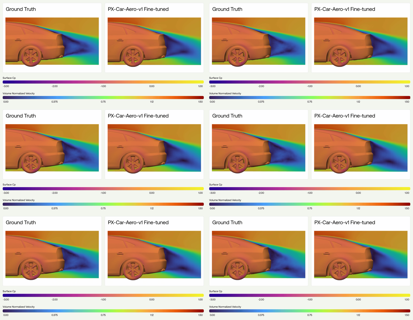
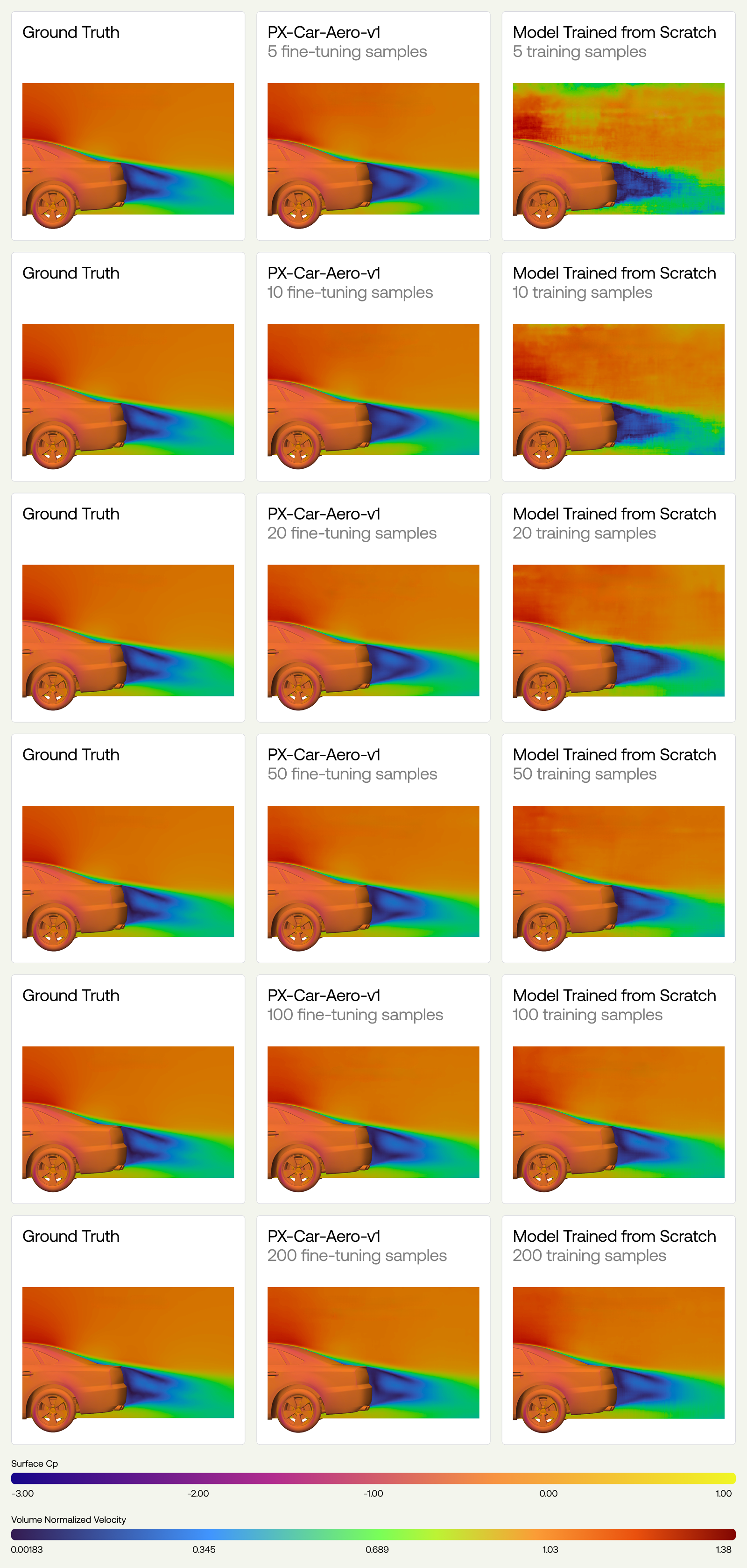
We can also see PX-Car-Aero-v1 adapt to a solver shift directly. As we increase the number of DrivAerML samples we fine-tune on, the refined features of the wake of the car emerge, and the volumetric pressure coefficient error reduces.

3.2 Fine-tuned LPMs can Capture the Complexity of Your Design Space, while Training from Scratch Struggles

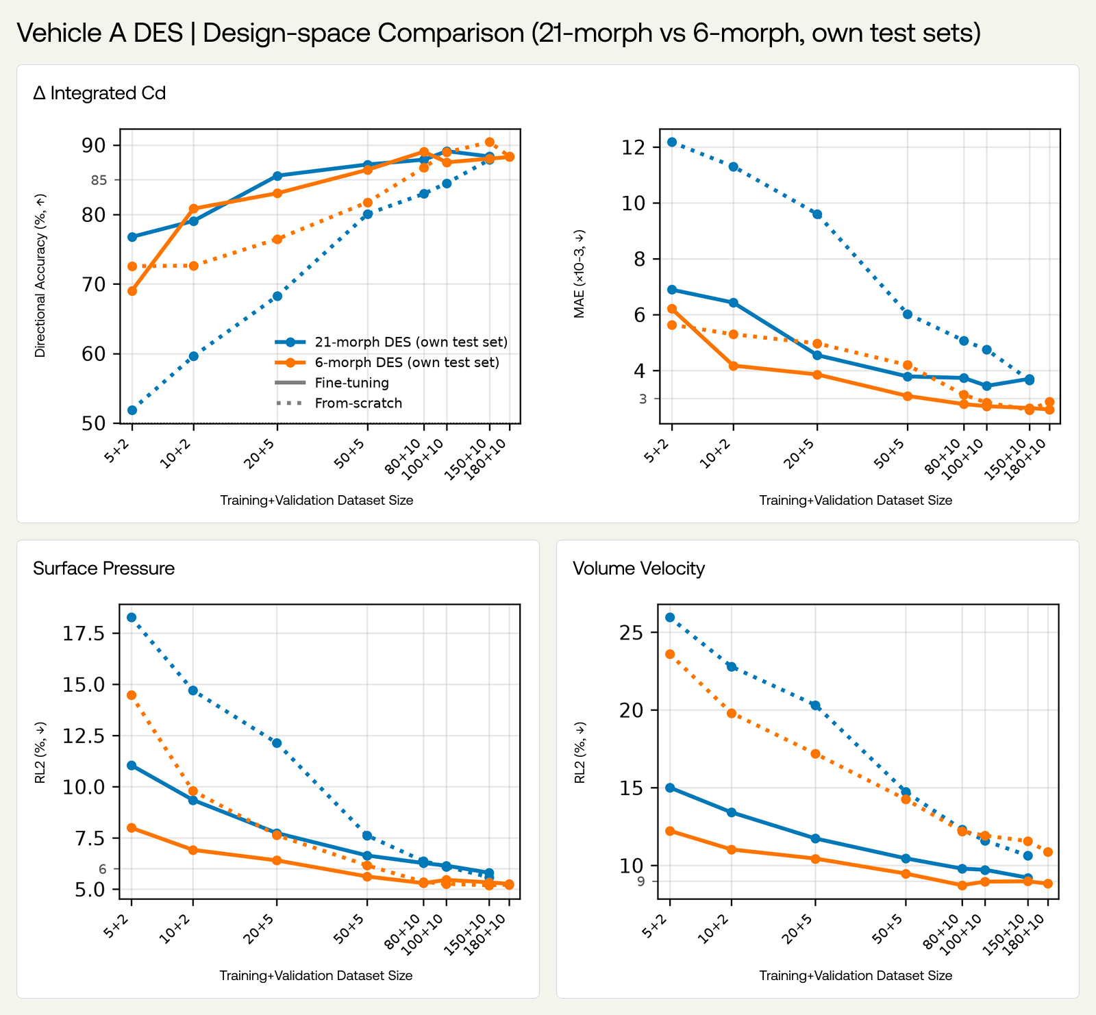
Fine-tuning scales effortlessly with design-space complexity. Comparing geometries morphed with 21 versus 6 unique parameters, the two fine-tuning curves nearly coincide, while training from scratch struggles at a low number of examples in the 21-parameter setting.

The six-parameter space restricts the design to the most influential architectural morphs: a handful of large body-shape changes, such as the overhangs and roof. The only difference between the two settings is the number of independent morph parameters used to generate the designs, so the comparison isolates how each method copes as the design space widens rather than as the geometry or solver changes. The pre-trained neural field absorbs the larger, harder design space at virtually no additional data cost. In contrast, training from scratch requires substantially more data as task complexity increases, catching up only at the largest data budgets. On the broader design space, it requires roughly 1.5× more data than on the narrower one. Pre-training, therefore, grows its advantage precisely where it matters most: on the larger, more complex design spaces that real-world industrial engineering problems demand.

3.3 Fine-tuning Performance Scales with Pre-trained Corpus Size

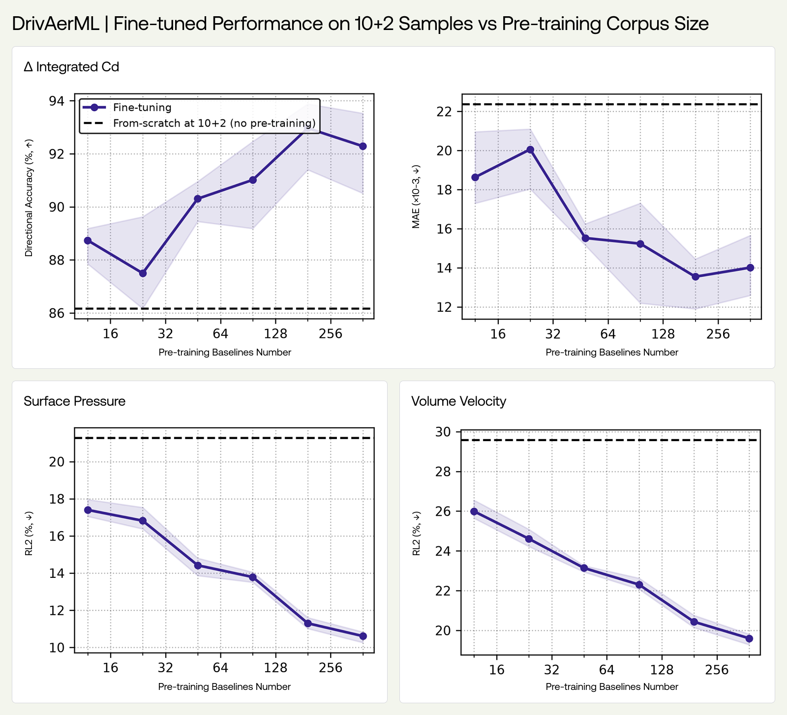
As our pre-training dataset continues to grow in size and diversity, so does the capability of the pre-trained model. The results presented so far use a fixed pre-trained model while varying the fine-tuning data budget. To understand how fine-tuning performance scales with the pre-training data size, we take pre-trained checkpoints built from 12 up to 384 baselines and fine-tune each on DrivAerML at a fixed small budget of 12 simulations (the 10+2 split).

Downstream performance improves with pre-training scale on every metric as the corpus grows from 12 to 192 baselines: directional accuracy rises from about 89% to 93%, delta CD MAE falls from 0.019 to 0.014, surface-pressure RL2 falls from about 18% to 11%, and volume velocity RL2 from about 26% to 20%. The drag metrics largely saturate by 192 baselines for this fine-tuning example, while the field metrics continue to improve. Even the smallest 12-baseline pre-training is well ahead of training from scratch at the same budget, where directional accuracy is 86%, surface-pressure RL2 is 21%, and volume velocity RL2 is 30%. While this is an indicative, preliminary result, we plan to develop a full set of fine-tuning scaling laws spanning a range of fine-tuning sample sizes and a broad set of use cases.

‍

4. The Road Ahead

The automotive LPM results above give us conviction that training on larger, more diverse datasets yields useful pre-trained models. Lower data requirements for adapting LPMs to new contexts drive down deployment costs for every use case and unlock capabilities in data-sparse applications.

We will continue to improve PX-Car-Aero-v1 by:

• moving to higher-fidelity DES simulations, prioritizing the most informative designs through active learning with a calibrated uncertainty quantification acquisition function applied to a pool of high-fidelity and generative geometries;
• continually advancing the model architecture;
• and applying active learning during downstream adaptation.

We are also exploring alternative pre-training strategies based on different fundamental paradigms. These include self-supervised pre-training, which combines broad geometry with low-fidelity synthetic physics to learn geometric representations that transfer to downstream physics tasks, and in-context learning as an alternative to the pre-train-then-fine-tune paradigm.

Meanwhile, we are expanding our portfolio of LPMs beyond automotive aerodynamics into other physics domains, including aeroelasticity for aircraft and turbomachinery. As the PhysicsX Data Factory continues to grow, so will the breadth and capability of our models. We are building dedicated pre-trained models for what we consider to be the most promising domains, or where we see immediate demand, while assessing whether a joint model spanning verticals confers advantages over narrower models.

As our pre-training datasets continue to grow and our models continue to improve, every new release will deliver stronger out-of-the-box performance and require less data to adapt to new high-complexity engineering problems.